Regression: Understanding What Covariates and Confounds Do in Adjusted Analyses

In observational studies, and occasionally in randomized controlled trials, as well, data are analyzed using linear, logistic, proportional hazards, and other models of regression. This article presents a brief, noncomprehensive explanation about variables, correlation, and regression and uses dummy data files to illustrate what happens when covariates and confounds are included in regressions.

Readers who are knowledgeable about statistics and research methods may wish to skip directly to the 3 examples discussed in this article. All readers will appreciate the points made in this article best if they run the regressions themselves; the dummy data files are provided as Supplementary Materials. Authors are also encouraged to read the articles cited in the references because these provide more detailed discussions on what is explained in this article.

Basic Concepts: Variables

Research is usually conducted to examine hypotheses, and hypotheses usually examine relationships between variables. A research study may include one or more independent variables (IVs), such as risk factors, and one or more dependent variables (DVs), such as the outcome(s) of interest. As an example, a study may examine whether gestational exposure to valproate (the IV) increases the risk of major congenital malformations in offspring (the DV). Or, a study may examine how antidepressant drugs and psychotherapy (IVs) reduce depression and suicidality (DVs) in adolescents with major depressive disorder. The IVs identified in these examples are the “IVs of interest” because they are part of the hypotheses being studied.^1,2

Research usually includes dozens of IVs beyond the IVs of interest; these IVs are the sociodemographic variables, clinical variables, and other variables that are relevant to the subject of study. Many of these IVs merely describe the sample so that the reader can understand to what population the findings of the study may be generalized. Others may be included in inferential statistical analysis because they have potential to influence the outcome; these variables are called covariates. Thus, covariates are IVs that are studied along with the IV of interest and are “adjusted for” when examining the effect of the IV of interest on the DV.³

As an example, we notice that words are produced by the mouth and that the mouth contains teeth. So, we decide to study whether the number of teeth (IV) that a preschooler’s mouth contains predicts the child’s vocabulary (DV). In this analysis, socioeconomic status is a possible covariate because preschoolers from higher socioeconomic strata may have better opportunities to learn new words; so, when examining the association between teeth and vocabulary, we must “adjust” the analysis for socioeconomic status. Enrollment vs no enrollment in preschool may likewise be included as a covariate in this analysis. A single analysis may include many covariates.

We also realize that older children have had more time and opportunity to learn words and that older children also have more teeth. We wonder whether our hypothesized relationship between number of teeth and vocabulary is explained by age. We therefore add age to our list of covariates in the analysis. Here, age is a confounding variable. In explanation, a confounding variable is a special kind of covariate; it is correlated with both the IV and the DV and can at least partly explain the association between the IV and the DV.^3,4

Basic Concepts: Correlation

Relationships between variables can be studied in many ways, such as by using correlation and regression. Correlation tells us the strength of relationship between variables, and regression quantifies the relationship.

As an example, we might find that there is a strong positive correlation between the number of teeth in the mouth and the number of words a preschooler knows; the correlation coefficient, r, is (for example) 0.72. We are impressed, because the maximum value for a (positive) correlation is 1.00, and because we seldom observe r values >0.80 in real world research. We are also impressed because the square of the correlation coefficient gives us the variance explained in the DV, and because (0.72)² is 0.5184, or 51.84%; that is, in our fictitious example, teeth predict an impressive 52% of the variance in a preschooler’s vocabulary.

As a side note, variance is a technical concept that (in this example) quantifies the extent to which the vocabulary of individuals in the sample differs from the average of the sample. Less technically, variance quantifies the scatter in vocabulary scores. The maximum explainable variance is 100%. In real life research, even with a whole bunch of IVs, we are seldom able to explain more than 70%–80% of the variance in a DV.

As a second side note, the variance in Vocabulary explained by Teeth is identical to the variance in Teeth explained by Vocabulary. This is because correlation does not imply cause and effect, and so does not specify a direction; for all we know, in our fictious study, increasing vocabulary can stimulate the growth of new teeth. This sounds absurd in our deliberately absurd example but can be a source of much misunderstanding in real research where cause-effect relationships are sought in correlation and regression analyses.

As a final side note, correlation between 2 variables, or bivariate correlations, are also called zero order correlations. In such correlations, the variance that each variable explains in the other is called shared variance.

Basic Concepts: Bivariate Linear Regression

Regression uses the study data to derive a formula that allows us to predict the value of a DV (eg, the outcome) given the values of one or more IVs (eg, the risk factor[s]). In this derived formula, each IV is assigned a coefficient that tells us by how much the value of the DV changes per unit change in the IV; in our fictitious study, we might find that with each additional tooth, a child’s vocabulary increases by 100 words.

There are many kinds of regression. One is bivariate linear regression, where the relationship between one IV and one DV (2 variables; hence “bivariate”) is modelled as a straight line. We know from our schooldays math that, on a graph, the equation for a straight line is as follows:

This equation is the simplest example of a regression equation. In this equation, y is the value of the DV for a subject, x is the value of the IV for that subject, and a and b are constants the values of which are the same for all subjects.

As a side note, in the equation, a is the intercept; that is, the value of y when x = 0. So, a is the point at which the regression line meets the y-axis. The value of the intercept is an indication of the extent to which y does not depend on x. In the equation, b is the slope of the regression line; the larger the value of b, the greater the value of y, and hence the steeper the slope.

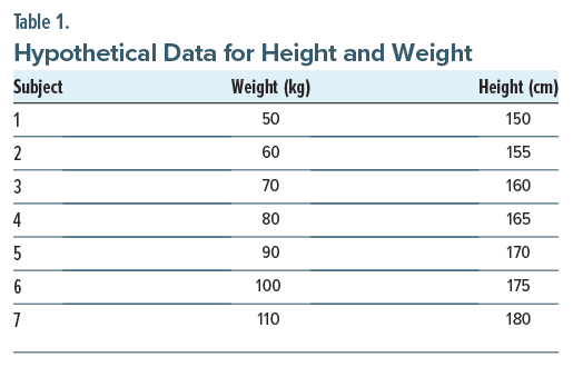
Table 1 presents the weight and height data for 7 imaginary subjects. If we model these data using linear regression, with the intent to predict a subject’s height (y) given that subject’s weight (x), we get the following regression equation:

We can confirm that this equation is correct when we use it to find the value for height by substituting for x any value for weight in Table 1.

As a side note, if we use this equation to estimate height from values of weight that lie outside the range of weights in Table 1, we might get absurd values for height. This illustrates the dangers of extrapolation beyond the range of observed values.

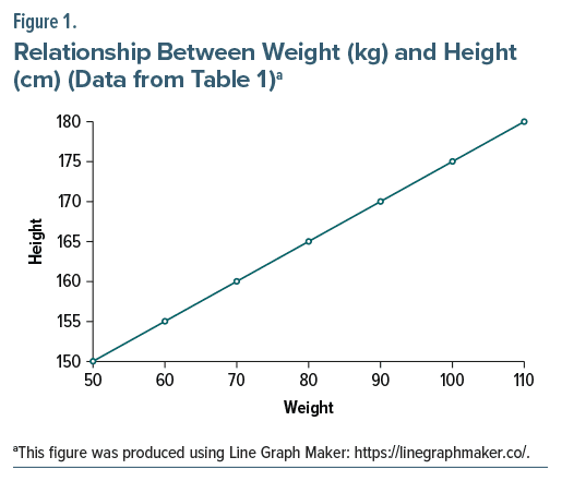
The data in Table 1, when plotted on a graph, lie along a straight line; this is the regression line (Figure 1). Because the data in Table 1 were idealized, all the data points lie on the regression line. In real life, however, the display of our x and y variables is a scattergram with the data points untidily scattered on the graph sheet; the regression line is therefore mathematically derived as the line of least squares.

As a technical note, in the scattergram of our data points for the x and y variables, the distance is measured between each data point and a straight line that is drawn through the scattergram. This distance (also known as the residual) is squared and the squares are averaged. The straight line that yields the least value for the average is the line of least squares, or the regression line. Expressed more simply, the regression line is the straight line passing through the scattergram that is closest to all the data points.

Basic Concepts: Multivariable Linear Regression

Multiple or multivariable linear regression differs from bivariate linear regression in that it includes more than one IV. So, the regression equation is as follows:

In this equation, y is the DV, x₁, x₂, x₃ … x_n are the first, second, third, … nth IVs, a is a constant (the intercept), and b₁, b₂, b₃ … b_n are the constants (slopes) for the IVs x₁, x₂, x₃ … x_n.

In multivariable regression, the line of least squares becomes multidimensional and can no longer be visualized or plotted on a 2-dimensional graph. Nevertheless, the concept is mathematically definable.

The Regression Coefficients

The b values are called b, B, or even β weights or coefficients with different terms used in different statistical articles, texts, and software programs. There are 2 values for these coefficients. One is the raw value and the other is the standardized value.

The raw value is usually presented as a b or B value; the standardized value is usually presented as a β or standardized β value. The raw value b_n tells us by how much y (the DV) changes per unit change in x_n (IV); the standardized value β_n tells us by how many standard deviations y (the DV) changes per SD change in x_n (IV). Note that each b or β is relevant only to its x; that is, the b₁ value applies to x₁, the b₂ value applies to x₂, and so on, as in the formula in the previous section.

Because the b values are in the units of the corresponding x variable, b values cannot be numerically compared across IVs. However, the (standardized) β units are in units of standard deviation and so these βs can be compared across IVs to allow us to understand which IV is influencing the DV more. Readers are reminded that the larger the value, the greater the effect. Readers may also note that a b value that is positive indicates that its IV is positively correlated with the DV whereas a b that is negative indicates that its IV is negatively correlated with the DV.

R, R², and Adjusted R²

After the multivariable regression is run in the statistical program and the constant a is derived, and the b coefficients identified for each x variable, the predicted y value for each subject can be calculated using the regression formula (this does not actually need to be done, though) and compared with the actual value of y for that subject. The difference between the actual and the predicted values for a subject is the “residual” for that subject. We had encountered this term earlier; the ideal regression line or line of least squares is the line which has the lowest sum (or average) of residuals.

The correlation between the actual values of y and the predicted values of y is represented by R; R (upper case), or the multiple correlation coefficient, is to multivariable regression as r (lower case) is to bivariate regression. R² in multivariable regression represents the variance in the DV explained by all the IVs in the equation much as r² in bivariate regression represents the variance in the DV explained by the single IV in the equation. More important than R², though, is adjusted R², or aR². The adjustment applies a correction to R² for each IV in the equation; the larger the number of IVs, the greater the correction. Among the R, R², and aR² values that are included in the statistical software output, only aR² is of interest to us.

In the rest of this article, we will look at how IVs influence DVs before and after covariates and confounds are added.

Example 1

We examine data from an entertaining study in which 48 young men were timed in a 100 m sprint. There were 12 men who ran without assistance; their timings lay in the 13.9–14.1 s range (mean, 14.0 s). There were 12 men who drank a large cup of coffee an hour before the time trial; their caffeine-assisted timings lay in the 13.5–13.7 s range (mean, 13.6 s). There were 12 men who did not drink coffee but who were unexpected chased by a bull; their bull-assisted timings lay in the 13.5–13.7 s range (mean, 13.6 s). Finally, there were 12 men who drank coffee as well as were chased by a bull; their caffeine- and bull-assisted timings lay in the 13.5–13.7 s range (mean, 13.6 s). The data are summarized in Table 2. The complete (raw) dataset is presented in the Supplementary File JCPRegression1.xlsx; the first worksheet presents the data and the second worksheet, the coding details.

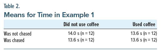
From the above, we observe that, regardless of its source, assistance was associated with 100 m sprint timings that were a mean of 0.4 s less than the mean of the unassisted timings. We also observe that having 2 sources of assistance was no better than having 1 source of assistance; perhaps, there was a ceiling effect to how fast those young men could run.

Note that we do not infer cause-effect relationships. That is, we do not say that drinking coffee or being chased by the bull improved timings; rather, we say that such assistance was associated with faster timings. We use our words carefully because we did not study the same men in 4 different conditions (unassisted, caffeine assisted, bull-assisted, and doubly assisted) nor were the men randomized to these 4 groups (but in the rest of this article, for simplicity, phrasing will imply cause and effect).

Now, let us see what happens when we run the data in bivariate and multivariable regressions (readers are strongly encouraged to run the regressions themselves, using any appropriate statistical software and the JCPRegression1.xlsx data file, to better follow what is discussed; however, this is not mandatory).

We start with a bivariate regression that examines how drinking coffee affects the sprint timings. The IV is Coffee, and the DV is Time. We run the regression and observe from the statistical software regression output that Coffee explains 25.7% of the variance in Time (aR² = 0.257); this is a modest value but is impressive enough given that Coffee is a single variable. The variance explained is statistically significant (F = 17.25, df = 1,46, P < .001), and the β coefficient for Coffee (–0.522) is statistically significant, indicating that drinking coffee significantly improves sprint timing.

The regression equation, obtained from the regression output, is as follows:

Coffee was coded as 0 = did not drink coffee and 1 = did drink coffee. So, substituting 0 for Coffee in this equation tells us that, without coffee, the timing of the average sprinter was 13.8 s (value of the intercept). This surprises us because we know that the average unassisted sprint time was 14.0 s; how did it become 13.8 s?

The answer is that, among the 24 sprinters who did not drink coffee, the average of 12 sprinters (no coffee, not chased) was 14.0 s and the average of the other 12 (no coffee, chased by the bull) was 13.6 s; so, the grand mean for the no coffee condition was 13.8 s.

There is another surprise in this regression equation. The (unstandardized) b coefficient for Coffee is −0.2. That is, for every 1 unit increase in Coffee, Time decreases by a mean of 0.2 s. Because Coffee has only 2 values, 0 and 1, it means that moving from no coffee to drinking coffee reduces the mean sprint time by 0.2 s. We are astonished because we knew, a priori, that drinking coffee actually improved timings by a mean of 0.4 s.

The explanation is that, among the 24 sprinters who drank coffee, whether or not they were chased, the mean sprint time was 13.6 s; but among those who did not drink coffee, as we noticed above, the mean sprint time was 13.8 s. So, the apparent benefit with coffee was only 0.2 s.

The 2 surprises discussed above illustrate a large learning point. The regression equation fits the data, but the results are misleading because, if there is something going on in the data that we don’t know about, we don’t put it into the regression, and so we don’t get an accurate picture. The “something” in this bivariate analysis is Chased, a covariate. As a generalization, in clinical research, regression models that associate IVs with a DV may be inaccurate if we fail to identify and include relevant covariates.

What happens if, instead of running a bivariate regression between Coffee and Time, we run the regression between Chased and Time? The findings are exactly the same because Chased and Coffee had exactly the same effects in the sample. So, the learning point is again the same.

Bivariate regressions yield unadjusted estimates. The b values are the unadjusted estimates. We now recognize that unadjusted estimates can be misleading, and so we run the regression with both Coffee and Chased as IVs and with Time as the DV. This becomes a multivariable regression because there is more than 1 IV.

As a side note here, if Coffee is our IV of interest, then Chased is the covariate that is adjusted for. If Chased is the IV of interest, Coffee becomes the covariate that is adjusted for. If we no idea what either of these IVs is doing in the data but want to find out, then both are IVs of interest in an exploratory regression.

We observe from the multivariable regression statistical output that Coffee and Chased together explain 52.5% of the variance in Time (aR² = 0.525); that’s impressive for just 2 variables. The variance explained is statistically significant (F = 27.00, df = 2,45, P < .001), and the β coefficients for Coffee (−0.522) and Chased (−0.522) are statistically significant, indicating that drinking coffee and being chased each significantly improved sprint timing.

The multivariable regression equation is as follows:

This multivariable regression tells us that the 2 variables together explain more of the (aR²) variance in timings than either variable alone. We also see that the b and β coefficients are unchanged, indicating that neither variable undercuts the contribution of the other (this is because the correlation between Coffee and Chased is 0; readers are encouraged to run the correlation to see for themselves).

Substituting 0 and 1 (in different combinations) for Coffee and Chased in this equation tells us that sprinters who did not drink coffee and were not chased ran the 100 m in a mean of 13.9 s; that those who drank coffee but were not chased had a mean timing of 13.7 s; that those who were chased but did not drink coffee had a mean timing of 13.7 s; and that those who drank coffee as well as were chased had a mean timing of 13.5 s. The values are again not what we expect from what we know about the data, and the b coefficients are also not what we expect from what we know.

Taking a step back, we realize that had we analyzed these data using 2-way analysis of variance, we’d have obtained F values for a main effect for Coffee, a main effect for Chased, and a Coffee×Chased interaction. Given that analysis of variance and linear regression are related concepts, we decide to create an interaction term (Inter) in the data.

For readers who are also running the regressions while following this discussion, this new variable is represented by “Inter” in the data file, and the values for Inter were created by multiplying the values of Coffee and Chased.

We now run the multivariable regression again, this time with Coffee, Chased, and Inter as the IVs and with Time as the DV. We observe from the regression output that Coffee, Chased, and Inter explain 80.6% of the variance in Time (aR² = 0.806); that’s a very impressive proportion of the variance explained for any multivariable regression. The variance explained is statistically significant (F = 66.00, df = 3,44, P < .001), and the β coefficients for Coffee (−1.044), Chased (−1.044), and Inter (0.905) are statistically significant.

The new multivariable regression equation is as follows:

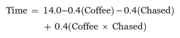
Readers may now check for themselves and confirm that the new equation fits the data; the b coefficients are correct, and the value for each of the 4 conditions is correct when the appropriate substitutions are made for Coffee and Chased in the formula.

So, another important learning point in Example 1 is that interaction terms also contribute to variance explained in the DV, and including the interaction term improves the fit of the regression equation to the data. Readers who are puzzled about where the interaction came from will find the answer in Table 2. If the means are plotted on a graph, the interaction is evident from the differing slopes of the lines.⁵

Here is a summary of what we saw in Example 1. We had 2 IVs. The correlation between the IVs was zero. Each IV explained the same proportion of the variance in the DV, and there was no additive effect for an individual subject when the IVs were both present. We found that including both IVs in the same regression increased the proportion of the variance in the DV explained without diminishing the values of the b coefficients that were observed in separate (bivariate) regressions. We observed that we cannot interpret the results of the regression correctly when we leave out a covariate that significantly influences the DV. We observed that including the covariate also did not correctly describe the model. We found that including an interaction term along with the IVs best described the model.

Example 2

The data in the Supplementary File JCPRegression2.xlsx are the same as those in Example 1 but with (only) 2 differences. First, drinking coffee had a smaller effect on the sprint timings. Second, sprint timings associated with both drinking coffee and being chased were slightly better than those associated with either condition alone. That is, the 2 conditions appeared to display a small additive effect (Table 3). Drinking coffee continued to show zero correlation with being chased.

Readers are again (though not mandatorily) encouraged to run the regressions and view the results. Coffee explained 22.3% of the variance in sprint timings; Chased explained 53.0% of the variance; Coffee and Chased together explained 77.0% of the variance; and adding the Coffee × Chased interaction term to Coffee and Chased explained 82.9% of the variance. All of these 4 regressions explained statistically significant proportions of the variance in Time.

The b coefficients were −0.2 and −0.3 for Coffee and Chased, respectively, with Time as the DV, and the coefficients were the same when these IVs were examined in separate (bivariate) regressions as well as when they were examined together in the same multivariable regression. The β coefficients also remained the same. However, the b coefficients were −0.3 and −0.4, respectively, when the interaction term was added to the regression, which, along with the intercept, reflected a good fit of the data (Table 3).

In summary, in Example 2, the correlation between the IVs was zero. The IVs explained different proportions of the variance in the DV and together had a small additive effect. Including both IVs in multivariable regression expectedly increased the proportion of the variance in the DV explained. However, despite the differences in the effects of the IVs and despite the additive effects, including both IVs in the regression did not diminish the values of the b and β coefficients observed in the separate (bivariate) regressions. Adding the interaction term yielded the best fit for the data.

Example 3

The data in the Supplementary File JCPRegression3.xlsx describe much the same study as in Examples 1 and 2. The differences are that the sample size has increased, drinking coffee has a smaller effect than being chased, and drinking coffee does not add to the effect of being chased (Table 4). Importantly, the correlation between Coffee and Chased, although small and not statistically significant (r = 0.167, P = .20), is no longer zero.

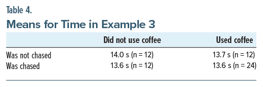
Running the regressions, as before, coffee alone explained 20.4% of the variance in sprint timings; Chased alone explained 48.0% of the variance; Coffee and Chased together explained 60.1% of the variance; and adding the Coffee× Chased interaction term to Coffee and Chased explained 77.1% of the variance. All of these were statistically significant.

In independent (bivariate) regressions, the b coefficients were −0.167 and −0.25 for Coffee and Chased, respectively, with Time as the DV; however, when Coffee and Chased were included in the same regression, the b coefficients dropped to −0.129 and −0.229, respectively; the β coefficient values also fell. But, when the interaction term was included, the b coefficients rose to −0.3 and −0.4, respectively, which reflects what is seen in the data (Table 4).

Why did the values of the b (and the associated β) coefficients decrease in the adjusted (multivariable) analysis? The answer is that whenever IVs are correlated, they share variance; this was explained in the Correlations section, early in this article. This shared variance is removed when the IVs are regressed together, leaving b coefficients that reflect the unique variance in the DV that each IV explains. The greater the correlation between IVs, the greater the shared variance removed, and hence the greater the fall in value of the b coefficients. One might therefore expect that adjusting for confounds in regression could result in a substantial loss of explanatory power, and even loss of statistical significance, of IVs. This is because, by definition, confounds are variables that are correlated not only with the DV but also with the IV of interest.^3,4

In summary, in multivariable analyses, when IVs are even weakly and nonsignificantly correlated, including both/all in a multivariable regression increases the overall variance explained but reduces the b and β coefficients that they display in bivariate regressions.

Take-Home Messages

Although this article explains what happens in unadjusted (bivariate) and adjusted (multivariable) linear regressions when there are just 2 IVs, the conclusions can be generalized to multivariable regressions that include many IVs. When important IVs (covariates, confounds), for whatever reason, are not included in regressions, the included IVs explain less of the variance in the DV. More importantly, the relationships between the included IVs and the DV are inaccurately modelled. Including interaction terms between IVs can improve the model whether the IVs are intercorrelated or not. When IVs are intercorrelated, such as when one is a confounding variable, although their net effect in multivariable regression may explain a greater proportion of the variance in the DV, their individual b and β coefficients decrease in proportion to the shared variance that is removed. This is why variables that were (perhaps deservedly) statistically significant in unadjusted analyses sometimes lose statistical significance in adjusted analyses. Readers may find it useful to keep these points in mind when running regressions on their data or when reading studies that present their results through regressions.

Parting Notes

Whereas concepts were explained in this article using linear regression, the concepts can also apply to other forms of regression. For excellent and comprehensive discussions on regression, from enumeration of assumptions to understanding of results, readers are encouraged to refer to standard statistical texts.^6,7

Article Information

Published Online: September 18, 2024. https://doi.org/10.4088/JCP.24f15573
© 2024 Physicians Postgraduate Press, Inc.
To Cite: Andrade C. Regression: understanding what covariates and confounds do in adjusted analyses. J Clin Psychiatry. 2024;85(4):24f15573.
Author Affiliations: Department of Psychiatry, Kasturba Medical College, Manipal Academy of Higher Education, Manipal, India; Department of Clinical Psychopharmacology and Neurotoxicology, National Institute of Mental Health and Neurosciences, Bangalore, India ([email protected]).
Relevant Financial Relationships: None.
Funding/Support: None.
Acknowledgment: I thank Dr David Streiner, PhD, FCAHS, CPsych (Ret), Emeritus Professor, McMaster University, Department of Psychiatry and Behavioural Neurosciences, Hamilton, Ontario, and Professor, University of Toronto, Department of Psychiatry, Toronto, Ontario, Canada, for his careful reading of this manuscript and for his support during its preparation.
Supplementary Material: Available at Psychiatrist.com